Using Postgres CREATE INDEX: Understanding operator classes, index types & more

Most developers working with databases know the challenge: New code gets deployed to production, and suddenly the application is slow. We investigate, look at our APM tools and our database monitoring, and we find out that the new code caused a new query to be issued. We investigate further, and discover the query is not able to use an index.

But what makes an index usable by a query, and how can we add the right index in Postgres?

In this post we’ll look at the practical aspects of using the CREATE INDEX command, as well as how you can analyze a PostgreSQL query for its operators and data types, so you can choose the best index definition.

How do you create an index in Postgres?

Before we dive into the internals, let’s set the stage and look at the most basic way of creating an index in Postgres. The essence of adding an index is this:

CREATE INDEX ON [table] ([column1]); 

For an actual example, let’s say we have a query on our users table that looks for a particular email address:

SELECT * FROM users WHERE users.email = 'test@example.com';

We can see this query is searching for values in the “email” column - so the index we should create is on that particular column:

CREATE INDEX ON users (email);

When we run this command, Postgres will create an index for us.

It's important to remember that indexes are redundant data structures. If you drop an index you don't lose any data. The primary benefit of an index is to allow faster searching of particular rows in a table. The alternative to having an index is to have Postgres scan each row individually ("Sequential Scan"), which is of course very slow for large tables.

Let's take a look behind the scenes of how Postgres determines whether to use an index.

Parse analysis: How Postgres interprets your query

When Postgres runs our query, it steps through multiple stages. At a high level, they are:

1. Parsing (see our blog post on the Postgres parser)
2. Parse analysis
3. Planning
4. Execution

Throughout these stages the query is no longer just text - it's represented as a tree. Each stage modifies and annotates the tree structure, until it's finally executed. For understanding Postgres index usage, we need to first understand what parse analysis does.

Lets pick a slightly more complex example:

SELECT * FROM users WHERE users.email = 'test@example.com' AND users.deleted_at IS NULL;

We can look at the result of parse analysis by turning on the debug_print_parse setting, and then looking at the Postgres logs (not recommended on production databases):

LOG:  parse tree:
DETAIL:     {QUERY 
	   ...
	      :quals 
	         {BOOLEXPR 
	         :boolop and 
	         :args (
	            {OPEXPR 
	            :opno 98 
	            :opfuncid 67 
	            :opresulttype 16 
	            :opretset false 
	            :opcollid 0 
	            :inputcollid 100 
	            :args (
	               ...
	            )
	            :location 38
	            }
	            {NULLTEST 
	            :arg 
	               ...
	            :nulltesttype 0 
	            :argisrow false 
	            :location 80
	            }
...

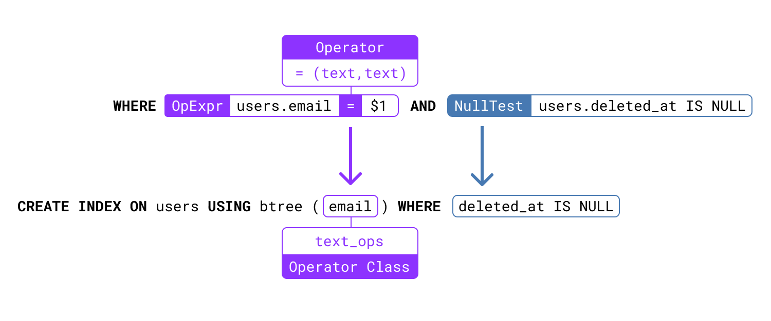
This format is a bit hard to read - let’s look at it in a more visual way, and with names instead of OIDs:

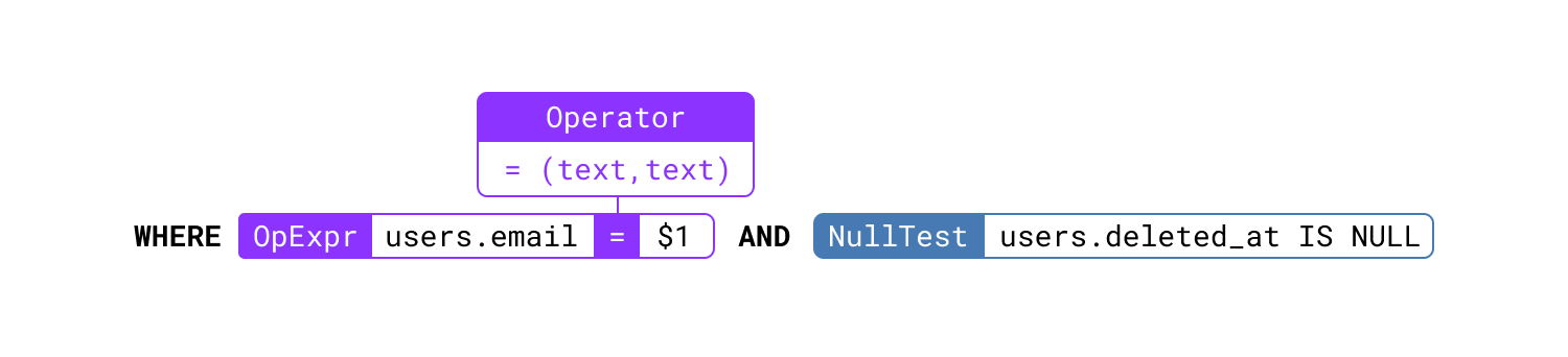
We can see two important parse nodes here, one for each expression in the WHERE clause. The OpExpr node, and the NullTest node. For now, let's focus on the OpExpr node.

Looking behind the scenes: Operators and data types

It's important to remember that Postgres is an object-relational database system. That is, it's designed from the ground up to be extensible. Many of the references that are added in parse analysis are not hard-coded logic, but instead reference actual database objects in the Postgres catalog tables.

The two most important objects to know about are data types and operators. You are most likely familiar with data types in Postgres, for example you have used them when specifying the schema for your table. Operators in Postgres define how particular comparisons between one or two values, for example in a WHERE clause, are implemented.

The OpExpr node represents an expression that uses an operator to compare one or two values of a given type. In this case you can see we are using the =(text, text) operator. This operator utilizes the = symbol as its name, and has a text data type on the left and right of the operator.

We can query the pg_operator table to see details about it, including which function implements the operator:

SELECT oid, oid::regoperator, oprcode, oprnegate::regoperator
  FROM pg_operator
 WHERE oprname = '=' AND oprleft = 'text'::regtype AND oprright = 'text'::regtype;

 oid |     oid      | oprcode |   oprnegate   
-----+--------------+---------+---------------
  98 | =(text,text) | texteq  | <>(text,text)
(1 row)

And if you really want to know what’s happening, you can look up the operator's underlying texteq function in the Postgres source:

/*
 * Comparison functions for text strings.
 */
Datum
texteq(PG_FUNCTION_ARGS)
{
    ...
    if (lc_collate_is_c(collid) ||
		collid == DEFAULT_COLLATION_OID ||
		pg_newlocale_from_collation(collid)->deterministic)
    {
        ...
    	result = (memcmp(VARDATA_ANY(targ1), VARDATA_ANY(targ2),
				  len1 - VARHDRSZ) == 0);
        ...
    }
    else
	{
        ...
        result = (text_cmp(arg1, arg2, collid) == 0);
        ...
    }
    ...
}

That function illustrates nicely how Postgres considers the collation to determine whether it can do a fast comparison that simply compares bytes, or whether it has to do a more expensive full text comparison. As we can see from the source, using a C locale for your collation can yield performance benefits.

Of course you can also define your own custom operators that work on your own custom data types. Postgres is extensible like that, and that’s actually pretty neat.

Operators are essential for creating the right index. The operator that is used by an expression is the most important detail, besides the column name, that indicates whether a particular index can be used.

You can think of operators as the "how" we want to search the table for values. For example, we may use a simple = operator to match values for equality against an input value. Or we may utilize a more complex operator, such as @@ to perform a text search on a tsvector column.

Finding the right index type

When you think of an index type, it's important to remember that it's ultimately a specific data structure that supports a specific, limited set of search operators. For example, the most common index type in Postgres, the B-tree index, supports the = operator as well as the range comparison operators (<, <=, =>, >), and the ~ and ~* operators in some cases. It does not support any other operators.

Let's say we have a tsvector column on our users table, and we use the @@ operator to search the column:

SELECT * FROM users WHERE about_text_search @@ to_tsquery('index');

Even if I create an index, it keeps doing a sequential scan:

CREATE INDEX ON users(about_text_search);

pgaweb=# EXPLAIN SELECT * FROM users WHERE about_text_search @@ to_tsquery('index');
                                 QUERY PLAN                                 
----------------------------------------------------------------------------
 Seq Scan on users  (cost=10000000000.00..10000000006.51 rows=1 width=4463)
   Filter: (about_text_search @@ to_tsquery('index'::text))
(2 rows)

This is because a B-tree index does not have the correct data structure to support text searches. There is no operator class that matches B-Tree indexes and the @@(tsvector,tsquery) operator.

Like earlier, thanks to Postgres extensibility, we can introspect the system to understand operator classes. Which index type can support the @@ operator on a tsvector column?

We can query the internal tables to answer this question:

SELECT am.amname AS index_method,
       opf.opfname AS opfamily_name,
       amop.amopopr::regoperator AS opfamily_operator
  FROM pg_am am,
       pg_opfamily opf,
       pg_amop amop
 WHERE opf.opfmethod = am.oid AND amop.amopfamily = opf.oid
       AND amop.amopopr = '@@(tsvector,tsquery)'::regoperator;

 index_method | opfamily_name |  opfamily_operator   
--------------+---------------+----------------------
 gist         | tsvector_ops  | @@(tsvector,tsquery)
 gin          | tsvector_ops  | @@(tsvector,tsquery)
(2 rows)

Looks like we need either a GIN or GIST index! We can create a GIN index like this:

CREATE INDEX ON users USING gin (about_text_search);

And voilà, it can be used by the query:

=# EXPLAIN SELECT * FROM users WHERE about_text_search @@ to_tsquery('index');
                                        QUERY PLAN                                         
-------------------------------------------------------------------------------------------
 Bitmap Heap Scan on users  (cost=8.25..12.51 rows=1 width=4463)
   Recheck Cond: (about_text_search @@ to_tsquery('index'::text))
   ->  Bitmap Index Scan on users_about_text_search_idx1  (cost=0.00..8.25 rows=1 width=0)
         Index Cond: (about_text_search @@ to_tsquery('index'::text))
(4 rows)

What's that tsvector_ops name we saw in the internal Postgres table?

That's how index types are linked to operators, using operator families and operator classes. For a given operator, there can be multiple different operator classes - an operator class defines how data is represented for a particular index type, and how the search operation for that index works to implement the operator used in a query.

Specifying operator classes during CREATE INDEX

For example let’s look at =(text,text), which is the operator used in an earlier query:

SELECT am.amname AS index_method,
       opf.opfname AS opfamily_name,
       amop.amopopr::regoperator AS opfamily_operator
  FROM pg_am am,
       pg_opfamily opf,
       pg_amop amop
 WHERE opf.opfmethod = am.oid AND amop.amopfamily = opf.oid
       AND amop.amopopr = '=(text,text)'::regoperator;

 index_method |  opfamily_name   | opfamily_operator 
--------------+------------------+-------------------
 btree        | text_ops         | =(text,text)
 hash         | text_ops         | =(text,text)
 btree        | text_pattern_ops | =(text,text)
 hash         | text_pattern_ops | =(text,text)
 spgist       | text_ops         | =(text,text)
 brin         | text_minmax_ops  | =(text,text)
 gist         | gist_text_ops    | =(text,text)
(7 rows)

You can see there is a default operator class (text_ops) that gets used when you don’t explicitly specify it - for text columns the default operator class is often all you need.

But there are cases where we want to set a particular operator class. For example, let's say we run a LIKE query on our database, and our database happens to use the en_US.UTF-8 collation - in that case, you will see the LIKE query is not actually able to use an index:

CREATE INDEX ON users (email);

pgaweb=# EXPLAIN SELECT * FROM users WHERE email LIKE 'lukas@%';
                                 QUERY PLAN                                 
----------------------------------------------------------------------------
 Seq Scan on users  (cost=10000000000.00..10000000001.26 rows=1 width=4463)
   Filter: ((email)::text ~~ 'lukas@%'::text)
(2 rows)

Generally, LIKE queries are challenging to index, but if you do not have a leading wildcard, an index can be created that works for them - but you need to either (1) use the C locale on your database (effectively saying you don’t want language-specific text sorting/comparison), or (2) use the text_pattern_ops operator class.

Let’s create the same index, but this time specify the text_pattern_ops operator class:

CREATE INDEX ON users (email text_pattern_ops);

pgaweb=# EXPLAIN SELECT * FROM users WHERE email LIKE 'lukas@%';
                                         QUERY PLAN                                         
--------------------------------------------------------------------------------------------
 Index Scan using users_email_idx on users  (cost=0.14..8.16 rows=1 width=4463)
   Index Cond: (((email)::text ~>=~ 'lukas@'::text) AND ((email)::text ~<~ 'lukasA'::text))
   Filter: ((email)::text ~~ 'lukas@%'::text)
(3 rows)

As you can see now the same LIKE query can use the index.

Now that we know our index type and operator class for our columns, let's look at a few other aspects of creating an index.

Specifying multiple columns when adding a Postgres index

One essential feature is the option to add multiple columns to an index definition.

You can do it simply like that:

CREATE INDEX ON [table] ([column_a], [column_b]);

But what does that actually do? Turns out it’s dependent on the index type. Each index type has a different representation for multiple columns in its data structure. And some index types like BRIN or Hash do not support multiple columns.

However with the most common index type, B-tree, multi-column indexes work well, and they are commonly used. The most important thing to know for multi-column B-tree indexes: Column order matters. If you have some queries that only utilize column_a, but all queries utilize column_b, you should put column_b first in your index definition. If you don’t follow this rule, you will end up with queries doing a lot more work because they have to skip over all the earlier columns that they can’t filter on. With GIST indexes on the other hand, this does not matter - and you can specify columns in any order.

Another decision to make is: Should I create multiple indexes, one for each column I’m querying by, or should I create a single multi-column index?

CREATE INDEX ON [table] ([column_a]);
CREATE INDEX ON [table] ([column_b]);
--- or
CREATE INDEX ON [table] ([column_a], [column_b]);

When looking at an individual query, the answer will almost always be: Create a single multi-column index that matches the query. It will be faster than having multiple indexes.

But if you have a larger workload, it may make sense to create multiple single-column indexes. Be aware that Postgres will have to do more work in that case, and you should verify what indexes actually get chosen by looking at your EXPLAIN plans.

Using functions and expressions in an index definition

Stepping back from specific index types for a moment: Postgres has a universal feature that applies to all index types, that's pretty useful: Instead of indexing a particular column's value, you can index an expression that references the column's data.

For example, we might typically compare our user email addresses with the lower(..) function:

SELECT * FROM users WHERE lower(email) = $1

If you were to run EXPLAIN on this, you would notice that Postgres is not able to use a simple index on email here - since it doesn’t match the expression.

But since lower(..) is what’s called a "immutable" function, we can use it to create an expression index, that indexes all values of email with their lower-case form:

CREATE INDEX ON users (lower(email));

Now our query will be able to use the index. Note that this does not work for all functions. For example, if you were to create an index on now(), it would fail:

CREATE INDEX ON users (now());

ERROR:  functions in index expression must be marked IMMUTABLE

Additionally, remember that expression indexes only work when they match the query. If we only have an index on lower(email), a query that simply references email won’t be able to use the index.

Specifying a WHERE clause to create partial PostgreSQL indexes

Let’s return to an example we saw at the beginning of the post - but now let’s look at the NullTest expression:

Here we are making sure we only get rows that are not yet marked as deleted by our application. Depending on your workload, this may be a very large number of rows that needs to be skipped over.

Whilst you could create an index that includes the deleted_at column, it would be quite wasteful to have all these index entries that you don’t actually want to ever look at.

Postgres has a better way: With partial indexes, you can restrict for which rows the index has index entries. When the restriction does not apply, the row won’t be saved to the index, saving space. And during query execution, this also acts as a significant time saver in many cases, since the planner can do a simple check to determine which partial indexes match, and ignore all that don't match.

In practice, all you need to do is add a WHERE clause to your index definition:

CREATE INDEX ON users(email) WHERE deleted_at IS NULL;

There are reasons why you may not want to do that though:

First, adding this restriction means that only queries that contain deleted_at IS NULL will be able to use the index. That means you may need two indexes, one with that restriction and the other without.

Second, adding hundreds or thousands of partial indexes causes overhead in the Postgres planner, as it has to do a more expensive analysis to determine which indexes can be used.

Using INCLUDE to create a covering index for Index-Only Scans

Last but not least, let’s talk about a more recent addition to Postgres: The INCLUDE keyword that can be added to CREATE INDEX.

Before we look at what this keyword does, let’s understand the difference between an Index Scan and an Index-Only Scan. An Index-Only Scan is possible when all data that is needed can be retrieved from the index itself - instead of having to fetch it from disk.

Note that Index-Only scans only work when the table has been recently VACUUMed - otherwise Postgres will need to check visibility too often for each index entry, and therefore does not opt to use Index-Only Scans, preferring an Index Scan instead in most cases.

Let's look at two examples - one query that matches an index fully, and one that does not (because of the target list):

CREATE INDEX ON users (email, id);

=# EXPLAIN SELECT id FROM users WHERE email = 'test@example.com';
                                     QUERY PLAN                                      
-------------------------------------------------------------------------------------
 Index Only Scan using users_email_id_idx on users  (cost=0.14..4.16 rows=1 width=4)
   Index Cond: (email = 'test@example.com'::text)
(2 rows)

=# EXPLAIN SELECT id, fullname FROM users WHERE email = 'test@example.com';
                                    QUERY PLAN                                    
----------------------------------------------------------------------------------
 Index Scan using users_email_id_idx on users  (cost=0.14..8.15 rows=1 width=520)
   Index Cond: ((email)::text = 'test@example.com'::text)
(2 rows)

Now, to get an Index Only Scan for the second query we can create an index that includes that column at the end - and that makes Postgres use an Index Only Scan:

CREATE INDEX ON users (email, id, fullname);

=# EXPLAIN SELECT id, fullname FROM users WHERE email = 'test@example.com';
                                           QUERY PLAN                                           
------------------------------------------------------------------------------------------------
 Index Only Scan using users_email_id_fullname_idx on users  (cost=0.14..4.16 rows=1 width=520)
   Index Cond: (email = 'test@example.com'::text)
(2 rows)

However, doing this has a few restrictions: It doesn’t work if you have unique indexes (since any column would modify what’s being checked for being unique), and it bloats the data stored in the index for searching.

For B-tree indexes the new INCLUDE keyword is the better approach:

CREATE INDEX ON users (email, id) INCLUDE (fullname);

This keeps the overhead for such additional columns slightly lower, works without problems with UNIQUE constraint indexes, and clearly communicates the intent: That you only added a column in order to support Index Only Scans.

This is a feature best used sparingly: Adding more data to the index means larger index values, which on its own can be a problem - it’s usually not a good idea to just add a lot of columns to the INCLUDE clause for an index.

Adding and dropping PostgreSQL indexes safely on production

I’ll end with a warning: Creating indexes on production databases requires a bit of thought. Not just which index definition to use, but also how to create them, and when to take the I/O impact of the new index being built.

The most important thing: Remember that Postgres will take an exclusive lock when you simply run CREATE INDEX, that will block all reads and writes to that table. That’s why Postgres has the special CONCURRENTLY keyword. When you create an index on a table on production that already has data, always specify this keyword:

CREATE INDEX CONCURRENTLY ON users (email) WHERE deleted_at IS NULL;

This is the same when dropping an index with DROP INDEX - adding CONCURRENTLY reduces the locking requirements slightly, making it faster to use this operation on production.

Conclusion

In this post you should have gotten a fundamental understanding of how operators and operator classes related to indexing, and why knowing these concepts is essential to creating the best index for complex queries. We also looked at a few complimentary features of the CREATE INDEX command, that are typically needed when reasoning about which index to create.

There are actually a few things we didn’t talk about: Adding indexes to specific tablespaces, using index storage parameters (especially useful for GIN index types!) and specifying the sort order for a particular column. I encourage you to take a further look at the Postgres documentation for these topics.

Share this article: If you liked this article you might want to tweet it to your peers.