EXPLAIN plan comparison

Here we first describe best practices for comparing EXPLAIN plans in Postgres, and then show the Plan Comparison feature in pganalyze.

In the course of analyzing query performance, you will typically need to compare EXPLAIN plans at some point. Plans can be obtained with the EXPLAIN command or with the auto_explain module.

Conceptually, one can either focus on either the overall plan shape or on the differences in execution metrics across matching nodes in two different plans.

Comparison basics

Generally speaking, there are no "good plans" and "bad plans" in Postgres. There are only plans that may be more or less appropriate for a given query. A sequential scan is more efficient and faster than an index scan when most of the data in a table is required to answer a query.

To compare two plans, it's important to understand why Postgres chooses a certain plan (which comes down to costs) and what alternate options are available.

Plan shape

Plans can vary significantly across different executions of the same query. The most impactful differences are generally in the scan nodes and join nodes selected for the plan. If you're trying to understand performance differences between plans, it's best to start with those nodes.

Plan metrics

EXPLAIN plans, especially ones gathered with the BUFFERS option, can be compared on a number of different metrics. Different metrics give different insights into the plans being compared:

• Cost: the cost to execute this node, as estimated by the planner
• Runtime: the total time it took to execute this node (requires auto_explain.log_timing for auto_explain plans)
• I/O Time: the total time this node spent performing I/O (requires track_io_timing on)
• Rows: the total rows returned by this node
• Buffers: the total number of pages read from either disk or the OS page cache (read) or found in shared_buffers (requires the BUFFERS option for EXPLAIN ANALYZE, or the auto_explain.log_buffers option for auto_explain)

All these metrics except row counts include the cumulative values from child nodes in standard EXPLAIN output.

Cost

This is a useful metric to understand the planner's "reasoning" for choosing what may be an inefficient plan. The planner determines cost based on statistics about the selectivity of query filters, information about the table, its data, and its indexes gathered by ANALYZE (both manual and through autovacuum); extended statistics; planner configuration settings; and derived estimates and heuristics.

Runtime

The execution time of the plan node, or the overall query. Note this excludes planning time and time spent waiting for locks. This is usually the most relevant metric overall: this determines query latency, and is ultimately what you will be trying to optimize.

I/O Time

The running time of expensive queries that read a lot of data from disk is usually I/O bound. Given the limited memory usage accounting available (see the Buffers section), actual time spent doing I/O is a good proxy for buffers read.

Note that this metric will vary depending on how much of the data needed by the query is already cached: if you are looking at auto_explain output, that will record how long the I/O took for that particular execution. But if you re-run the query with EXPLAIN ANALYZE, a different portion of the table data may now be in cache, so the I/O timing may not be comparable. You may want to review the buffer cache statistics for the tables involved to have a better understanding of differences in timing.

I/O timing is also useful if you can perform a cold cache test. To run a cold cache test, you'll need to restart Postgres and clear the OS page cache (see, e.g., these instructions for Linux).

Rows

Row count statistics can be useful to track down where a lot of data is discarded when evaluating a plan. Look for child nodes with a much larger row count than their parent nodes. Reading more data than necessary is a common query plan inefficiency. A common example of this is queries with a small LIMIT x and large OFFSET y: typically, these must read x + y rows, even though they only return x.

Buffers

Since I/O timing can be hard to test, you can instead look at the amount of data being processed. This requires the BUFFERS option to EXPLAIN or auto_explain.log_buffers for auto_explain.

The BUFFERS option will report buffers hit, read, dirtied, and written. It breaks this into three categories: shared, local, and temp. For comparing buffer usage for most queries, it's best to focus on the amout of table and temp table data read from disk or found in cache. This is represented by shared and local buffers hit and read (see the BUFFERS documentation linked above for details), and you can use this as a proxy for the I/O efficiency of the query plan.

Unfortunately, the BUFFERS option does not count unique buffer accesses: it counts the total number of accesses. Queries that read the same pages of data over and over (e.g., ones involving nested loop joins) can end up over-counting buffer usage.

Plan Comparison in pganalyze

You can access the Plan Comparison view from a few different places in pganalyze:

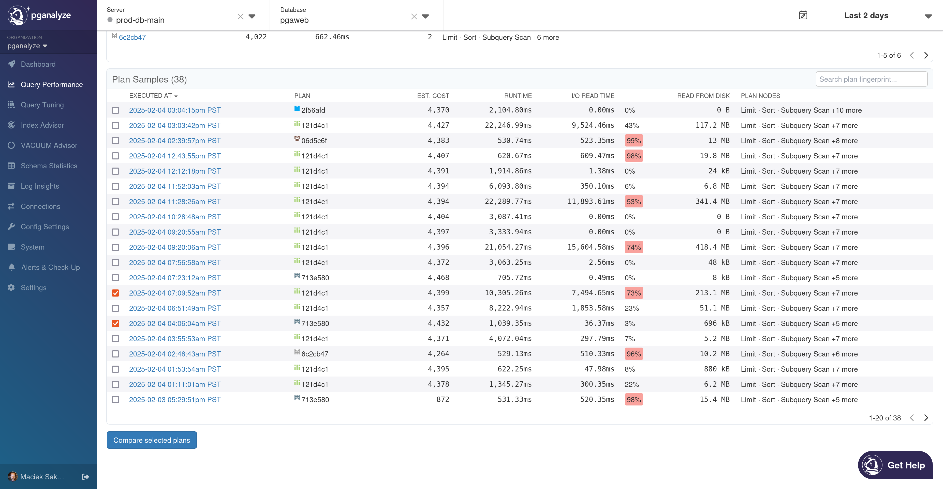
• the Plan Samples panel on the EXPLAIN Plans tab of the detail page for a particular query
• the Compare Plans button on the detail view for a specific plan
• the Overview page of a Query Tuning workbook

All of these have a list of plans with checkboxes. Select two and press "Compare Plans" to start a comparison.

The comparison itself consists of a diff-like view of the two different plan shapes, a metric selector and stats for the selected metric, and a sidebar for additional information:

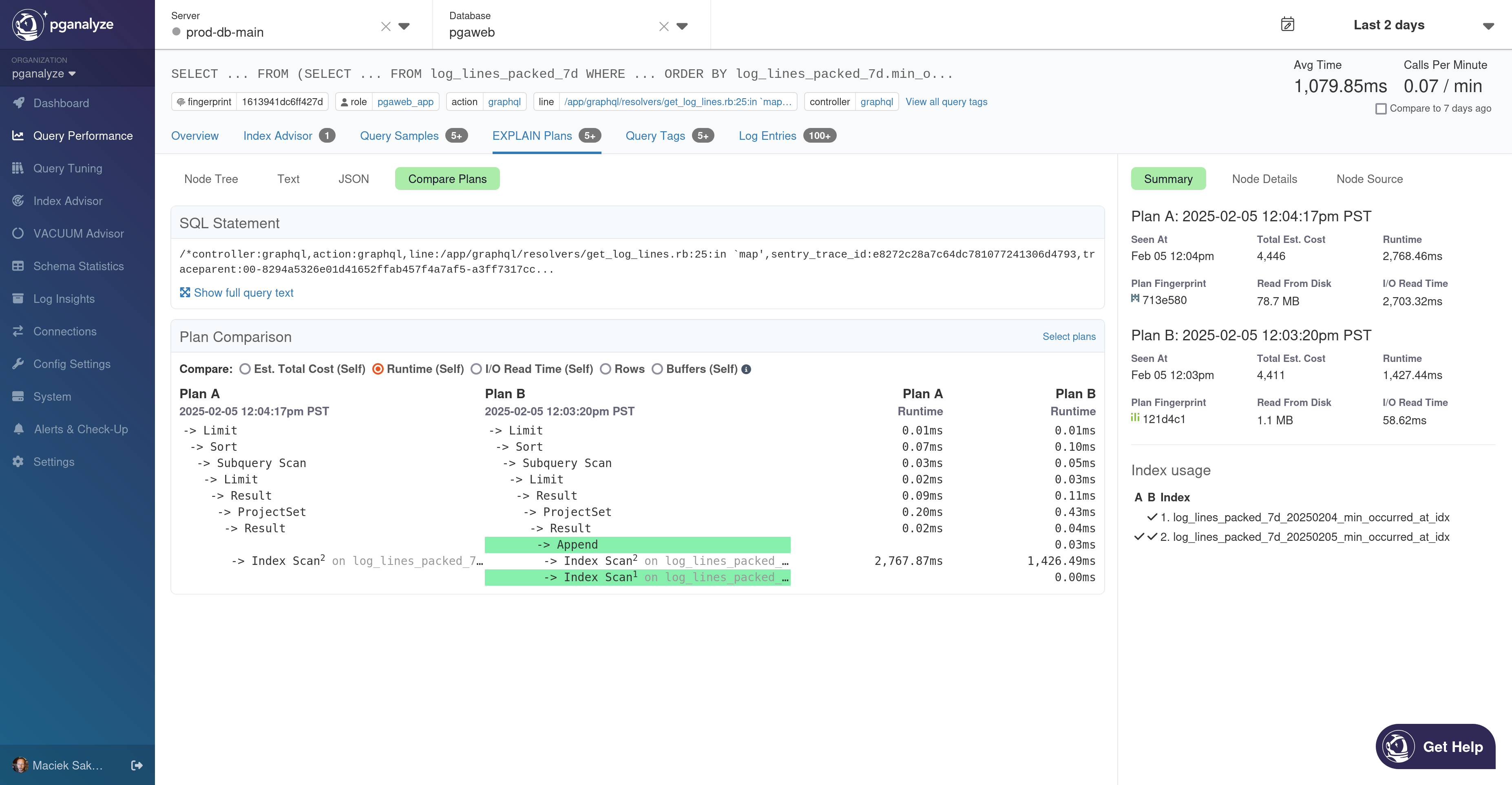
A summary of both plans is available in the sidebar on the right. Below the summary, there's a comparison of the index usage of these plans: all indexes used by either plan are listed, with a checkmark in the A column if the index is used by the first plan, and a checkmark in the B column if the index is used by the second plan. In the main plan diff view, indexes are referenced by footnote.

Nodes that scan tables, views, or set-returning functions include the table, view, or function name next to the node name in a lighter color. It may be truncated, but you can hover over the node to see the full name.

Subplans that are essentially executed separately in Postgres are split out into a separate section of the diff, below the main plan. Plan nodes that scan these subplans include the subplan name next to the plan node, just like table scans.

Clicking on a node in the diff view in either plan A or plan B will update the sidebar to show the details for that plan node. You can click Node Source to view the full JSON source for that node.

You can select a comparison metric at the top to see per-node comparisons according to that metric: all the metrics described above are supported.

Note that the Buffers metric is a combination of shared and local buffers hit and read, as in the Buffers section.